# For data manipulation
library(tidyverse)
# For reading subtitle files
library(srt)

### Use read_srt from {srt} to read the cats subtitle file.
cats <- read_srt("Cats_2019.srt")During the fear-filled weeks of March 2020, one of the brief reprieves of dread was when my friends and I watched Cats (2019) on Zoom. The film is a mess, a $95 million flop with a star-studded cast, filled with disconcerting CGI and with the thinnest of plots. But if watching Sir Ian McKellen as old Gus’s “Asparagus” the Theatre Cat, dressed as a CGI cat hobo getting startled while drinking milk from a saucer doesn’t distract you from the chaotic state of the world, I don’t think anything will.
To be fair to the movie, the source material didn’t give them much to work with. The stage production follows a group of cats called the “Jellicles” who must choose one of the cats to ascend to the “heaven side layer” to be reincarnated. Each song is just the cats being introduced to the audience. The stage production is the 4th highest-grossing musical ever. I don’t understand musicals. But I am fascinated when I don’t understand people’s attitudes or behaviors, whether it is why people have certain political opinions, vaccine skepticism, why individuals get in involved in criminal gangs, or why political leaders seize power through coups. Or in this case why people like the musical Cats. I can’t answer the question of why people like the musical Cats, but I can count how many times they mention the word ‘cats’ in Cats.
This tutorial will show some basics of using {tidytext} to work with textual data in some very basic ways.
Getting the data
The first thing we need to do to answer this question is to get the data. My first instinct was to look for a plain text script of the original 1981 stage production. Shockingly, I couldn’t find this online. I imagine Andrew Lloyd Webber is vigilant about protecting his Cats IP, it is after all the most successful musical of all time.
Then it struck me that I could use subtitles files from the film itself. These files are generally stored as .srt text files. One of the great features of R is that there is an amazing number of packages (over 18,000 on CRAN even more on GitHub). If you don’t know anything about R, packages are collections of tools that make doing certain tasks much easier. If you Google a specific task and “R package” chances are that you will find a package to help you with the task. For instance, last year I wanted to see if there were any packages that could read in images as vectors and then randomly change their hex codes to make glitchy images. As luck would have it there was an R package for that.
After a minute of googling, I found {srt}, a package that can read .srt files as a table with flags for start and end times along with the text of each subtitle line.
Exploring the dataset
To read in the data I am going to load {srt} along with the tidyverse collection of packages.
Here is what the data looks like. We have four columns, the n column denotes the subtitle number, start and end are time stamps for when the subtitles begin and end the 100th of a second. Lastly, the subtitle column has the text for each line.
| n | start | end | subtitle |
|---|---|---|---|
| 2 | 171.182 | 173.682 | ♪ Are you blind when you're born? ♪ |
| 3 | 173.684 | 175.953 | ♪ Can you see in the dark? ♪ |
| 4 | 177.688 | 179.688 | ♪ Can you look at a king? ♪ |
| 5 | 179.690 | 181.959 | ♪ Would you sit on his throne? ♪ |
| 6 | 183.828 | 186.829 | ♪ Can you say of your bite ♪ |
| 7 | 186.831 | 188.766 | ♪ That it's worse than your bark? ♪ |
| 8 | 190.001 | 192.835 | ♪ Are you cock of the walk ♪ |
| 9 | 192.837 | 194.870 | ♪ When you're walking alone? ♪ |
| 10 | 194.872 | 196.872 | ♪ When you fall on your head ♪ |
| 11 | 196.874 | 198.674 | ♪ Do you land on your feet? ♪ |
The counting of “cats”
Let’s start with some simple word count. For this I am going to use {tidytext}. To get frequency counts we need to prepare the data. First, I am using the unnest_tokens function which pulls out individual words and puts them each in their own rows. Then I am using the count function to get frequencies for each word. The final step in this process is to remove ‘stop words’. These are words that are common in speech but aren’t analytically interesting for this analysis (i.e. words like “the”, “and”, “I”, and “you”). Below is how the data looks in each stage of the process, ending with the summarized counts.
First, we use unnest_tokens. Here, we are pulling apart the subtitle column and giving each word its own row. The other identifying variables, the subtitle number and the time stamps remain the same. In the code below I am specifying the output and the input argument in unnest_tokens.
# For text manipulation
library(tidytext)

cats %>%
unnest_tokens(word, subtitle) | n | start | end | word |
|---|---|---|---|
| 2 | 171.182 | 173.682 | are |
| 2 | 171.182 | 173.682 | you |
| 2 | 171.182 | 173.682 | blind |
| 2 | 171.182 | 173.682 | when |
| 2 | 171.182 | 173.682 | you're |
| 2 | 171.182 | 173.682 | born |
| 3 | 173.684 | 175.953 | can |
| 3 | 173.684 | 175.953 | you |
| 3 | 173.684 | 175.953 | see |
| 3 | 173.684 | 175.953 | in |
Now that we have a dataframe where each row has a single word we can easily use count to get frequency counts for each word.
cats %>%
  unnest_tokens(word, subtitle) %>%
count(word, sort = TRUE)| word | n |
|---|---|
| the | 352 |
| and | 221 |
| a | 200 |
| i | 171 |
| you | 159 |
| to | 143 |
| of | 131 |
| jellicle | 97 |
| in | 93 |
| cat | 92 |
As you see, just counting the occurrences of each word isn’t super interesting because the English language is filled with articles, prepositions, pronouns, and conjunctions which are not (always) analytically relevant. When processing natural language data these words are referred to as ‘stop words’. In our simple analysis of counting the frequency of words, we really don’t need to know the frequency of various prepositions. Luckily, {tidytext} provides a dataset of stop words which makes it easy to filter them out using anti_join.
cats %>%
  unnest_tokens(word, subtitle) %>%
  anti_join(stop_words) %>%
count(word, sort = TRUE)| word | n |
|---|---|
| jellicle | 97 |
| cat | 92 |
| cats | 81 |
| jellicles | 34 |
| macavity | 25 |
| mistoffelees | 19 |
| magical | 18 |
| songs | 18 |
| life | 16 |
| time | 16 |
You’ll notice a few things here. An important thing to always remember when using R is that it does exactly what you tell it to do. Here, I told it to count all unique words, but since it is not actually understanding human language, it is counting unique combinations of characters. So, you’ll see that both singular and plural forms are counted as unique. For real text analysis it is common practice stem words, that is, reducing words into their base words. For example, programming, programs, programmed would all become program. For the purposes of this post, I am not going to stem all the words since we are only interested in the word cat. If you are interested in stemming Chapter 4 of Supervised Machine Learning for Text Analysis in R can give a more in-depth overview (along with more depth in every aspect of working with text data) To filter for just occurances of “cat” I am using ‘string_detect’ from {stringr}. This function takes a given string, in this case our ‘word’ column and looks for a pattern. The pattern takes regex (regular expression) which is string of characters that describes a search pattern. For me it is very unintuitive and I Google every time I have to use regex. In the pattern section the “\b” indicates word boundaries while ‘|’ is an operator for or.
cats %>%
  unnest_tokens(word, subtitle) %>%
  anti_join(stop_words) %>%
  count(word, sort = TRUE) %>%
filter(str_detect(word, "\\bcat\\b|\\bcats\\b|\\bcat's\\b"))| word | n |
|---|---|
| cat | 92 |
| cats | 81 |
| cat's | 3 |
In total adding up the variations of the word “cat” you can see that we have 176 mentions of “cat” in Cats (2019). The length of the film is 107.82 minutes which means there is an average of mention of ‘cats’ once every 36.76 seconds. But this average isn’t super informative, after all, words in musicals aren’t spread evenly throughout the entire length of the film. To understand this temporal dynamic, we need to build a new data frame. If you remember our cats data frame has a variable for the start and the end of when the subtitle appears, down to the 100th of a second. For our purposes, we don’t need to know when the subtitle ends but only where it appears on the screen.
cats %>%
# Renaming the `start` col as `time`
  rename(time = start) %>%
# Select just the time and subtitle col
  select(time, subtitle) %>%
# Count the number of cat mentions per subtitle
# Then get the cumulative sum of the count of cat mentions per subtitle
  mutate(cat_mentions = str_count(subtitle, "\\bcat\\b|\\bcats\\b|\\bcat's\\b"),
         cumulative_cat_mentions = cumsum(cat_mentions))
| time | subtitle | cat_mentions | cumulative_cat_mentions |
|---|---|---|---|
| 276.821 | ♪ Bounce on a tire ♪ | 0 | 6 |
| 278.890 | ♪ We can run up a wall ♪ | 0 | 6 |
| 280.791 | ♪ We can swing through the trees ♪ | 0 | 6 |
| 284.195 | ♪ We can balance on bars, we can walk on a wire ♪ | 0 | 6 |
| 288.232 | ♪ Jellicles can and Jellicles do ♪ | 0 | 6 |
| 290.968 | ♪ Jellicles can and Jellicles do ♪ | 0 | 6 |
| 293.804 | ♪ Jellicles can and Jellicles do ♪ | 0 | 6 |
| 296.007 | ♪ Jellicles can and Jellicles do ♪ | 0 | 6 |
| 298.809 | ♪ Jellicle songs for Jellicle cats ♪ | 1 | 7 |
| 300.778 | ♪ Jellicle songs for Jellicle cats ♪ | 1 | 8 |
| 303.080 | ♪ Jellicle songs for Jellicle cats ♪ | 1 | 9 |
| 305.750 | ♪ Jellicle songs for Jellicle cats ♪ | 1 | 10 |
| 308.287 | ♪ Can you sing at the same time in more than one key? ♪ | 0 | 10 |
With this dataset, we can make a quick chart showing the cummulative mentions of ‘cats’ in Cats (2019) over the duration of the film.
# For themes
library(hrbrthemes)
# For scales
library(scales)

ggplot(df, aes(x=time, y=cumulative_cat_mentions)) +
  geom_line( color="#69b3a2", size=2, alpha=0.9, na.rm = TRUE) +
  # X scale as time
  scale_x_time()+
  # Theme
  theme_ipsum()  +
  labs(title ="Cummulative mentions of 'cats' in Cats (2019)",
      x = "Film time",
       y = "Cummulative mentions of 'cats'",
      caption = "Chart by @JoeDNoonan")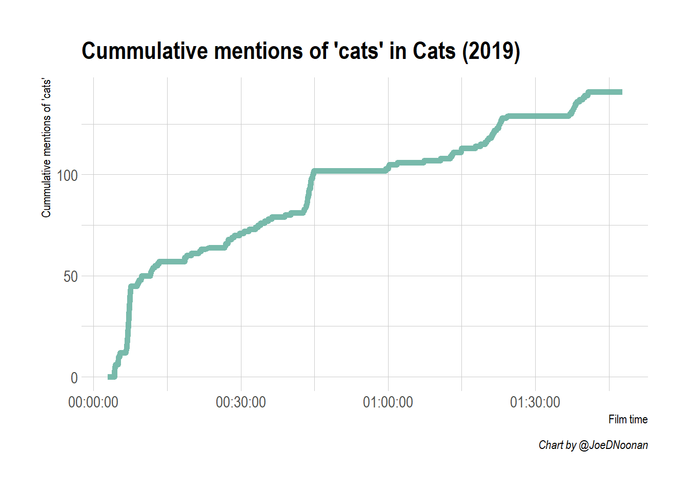
This chart is looking pretty good, but the line of the plot doesn’t start at the beginning of the x-axis. This is because our dataset actually only starts when the first subtitle is shown which is two minutes in. To fix this we can just make a blank data frame with a single row with and set all the numerical variables to 0 and subtitle to NA. Then we stack this blank dataframe on top of the original dataframe using rbind.
blank_df <- tibble(time = 0, subtitle = NA, cat_mentions = 0, cumulative_cat_mentions = 0)

ggplot(rbind(blank_df, df), aes(x=time, y=cumulative_cat_mentions)) +
  geom_line( color="#69b3a2", size=2, alpha=0.9, na.rm = TRUE) +
  scale_x_time()+
  theme_ipsum()  +
  labs(title ="Cummulative mentions of 'cats' in Cats (2019)",
      x = "Film time",
       y = "Cummulative mentions of 'cats'",
      caption = "Chart by @JoeDNoonan")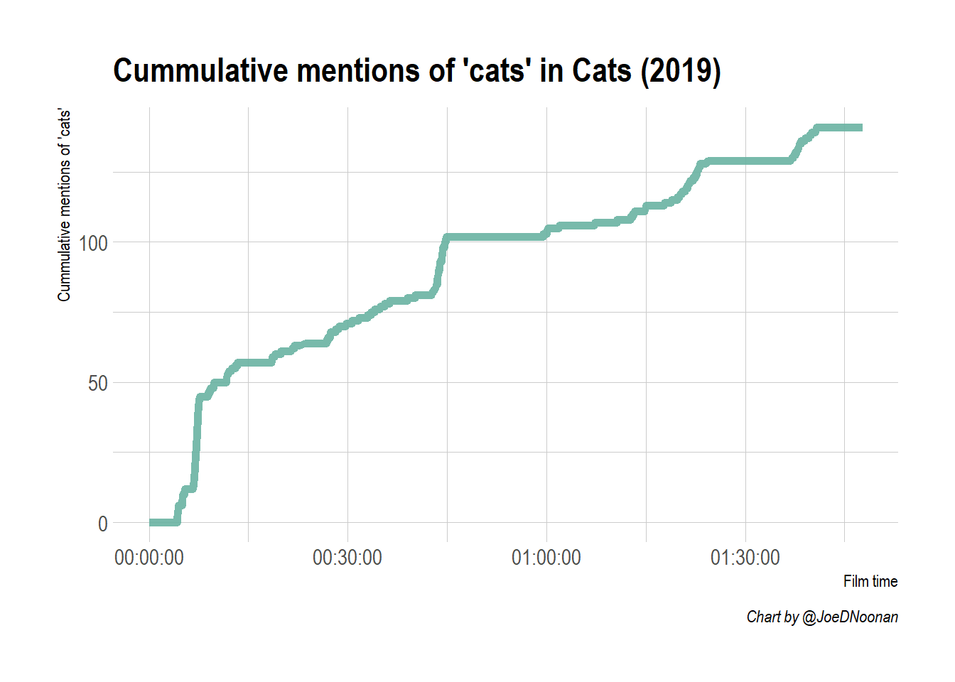
That looks better! You can see that there is a sharp rise early in the film, but it quickly slows down. With cumulative graphs, since they never go down, it can be difficult to see when occurrences increase. One way to visualize this differently is to show a simple bar plot with time broken into percentiles. To do this you need to create a new dataframe and create a new variable which bins the observations by time using ntile. Once you have created this variable you can use it to group and to summarize.
df2 <- df %>%
  mutate(time_percentile = ntile(time, n = 100)) %>%
  group_by(time_percentile) %>%
  summarize(cat_mentions = sum(cat_mentions))


ggplot(df2, aes(time_percentile, y=cat_mentions)) +
  geom_bar(stat="identity", fill="#69b3a2", size=2, alpha=0.9) +
  theme_ipsum() +
  labs(title ="Mentions of 'cats' in Cats (2019)",
      x = "Percentile bin of film time",
       y = "Mentions of cats",
      caption = "Chart by @JoeDNoonan")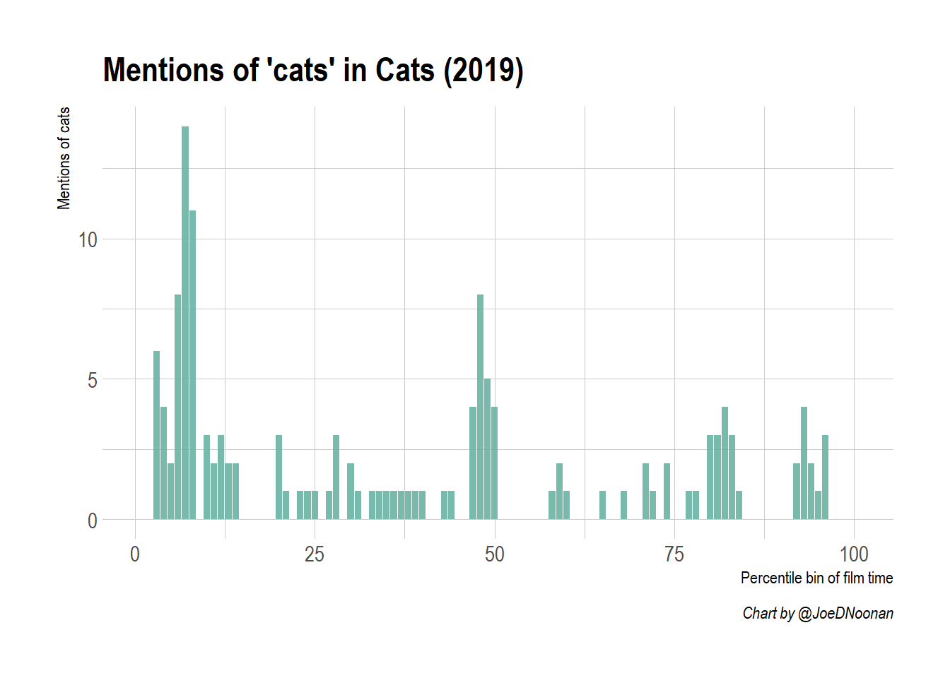
Here, it is pretty obvious that the first 10% of the film contains the highest frequency of cat mentions. This is probably because of the jarring, disorienting and frankly frightening first song “Jellicle Songs For Jellicle Cats” where the chorus has the cats hauntingly chanting “Jellicle Songs For Jellicle Cats”.
Conclusion
This blog post provided a quick overview of how to work with text analysis in R using .srt files as a data source. Textual data is fun but challenging data to work with. There is an abundance of textual data in the world but making sense of it requires a lot of cleaning and manipulation to make sense of it. If you are interested in learning more about working with textual data I would recommend the book Text Mining with R: A Tidy Approach which follows what I have shown here, or the tutorial to using quanteda, which is another package that has more advanced natural language processing tools.